The Kelly Allocation to a Single Security

The Kelly Allocation to a Single Security

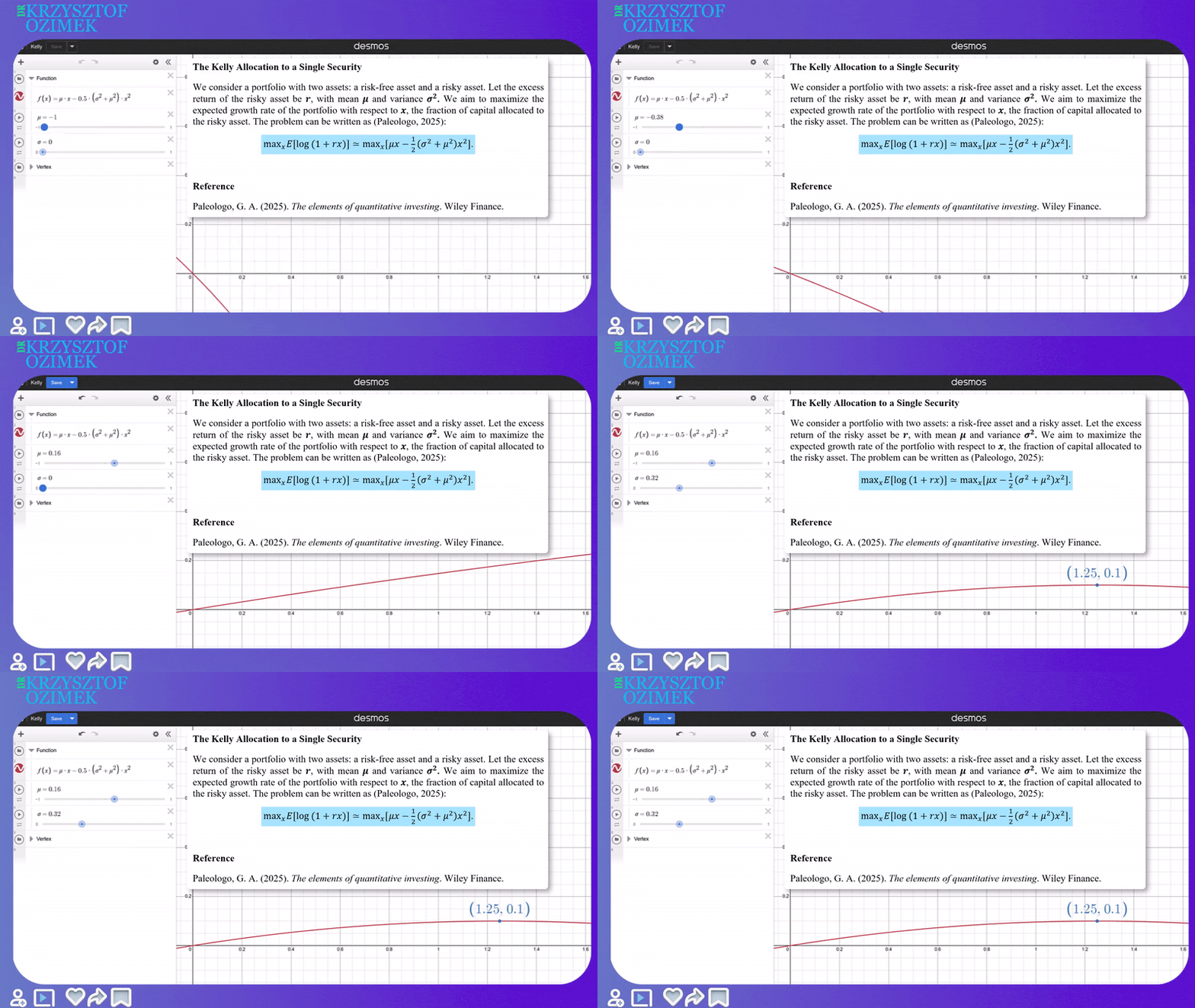
We consider a portfolio with two assets: a risk-free asset and a risky asset. Let the excess return of the risky asset be \(r\), with mean \(\mu\) and variance \(\sigma^2\). We aim to maximize the expected growth rate of the portfolio with respect to \(x\), the fraction of capital allocated to the risky asset. The problem can be written as (Paleologo, 2025):

\[ \max_x E[\log(1 + rx)] \approx \max_x \left[ \mu x - \frac{1}{2}(\sigma^2 + \mu^2)x^2 \right] \]

\[ x^* = \frac{\mu}{\sigma^2 + \mu^2} \]

For \(\mu = 0.16\) and \(\sigma = 0.32\):

\[ x^* = \frac{0.16}{0.32^2 + 0.16^2} = \frac{0.16}{0.1024 + 0.0256} = \frac{0.16}{0.128} = 1.25 \]

Does it seem counterintuitive that, with relatively high volatility being twice the expected return (32% versus 16%), the Kelly approximation prescribes investing all capital in the risky asset and leveraging an additional 25% to maximize portfolio growth?

The Kelly formula relies on \(\sigma^2\) as a complete description of risk. For a discussion of cases where variance-based risk measures can mislead, see the companion post on volatility.

Reference

Paleologo, G. A. (2025). The elements of quantitative investing. Wiley Finance.